
Software Demo: Epigenomic Browsers, CEpBrowser and Galaxy
Guest Instructor: Xiaoyi Cao, Bioengineering Department, University of California, San Diego
Index
When studying epigenomics at a large scale (usually genome-wide scale to look for specific epigenomic patterns or get a view of overall properties of certain epigenomic properties), a browser that not only provides quite a few epigenomic datasets, but also can lay them out with the genome in question and allow user to navigate through the genome will be very helpful. So here we will briefly introduce two browsers that have such data availability and visualization capacity.
This is a specialized UCSC Genome Browser collecting ENCODE and Roadmap Epigenomics data and is publicly available at http://www.epigenomebrowser.org. [1]
Users familiar with UCSC Genome Browser would find it easy to use this specialized version. The ENCODE data collected in the epigenome browser is grouped by data type (DNA methylation, histone, etc.) and contributors (Broad, SYDH and UW). the HMM chromatin states inferred from histone data for the cell lines can also be seen under the histone modification track.
Tracks can be shown in the browser directly by selecting the drop-menu for data type or in track details. Every track may have a "dense" display with a bed peak display. Custom tracks can be added by uploading compatible files or providing the URL.
Figure 1. GUI of Epigenome Browser from UCSC
WashU Epigenome Browser is developed by Wang lab at Washington University at St Louis. It can be accessed at http://epigenomegateway.wustl.edu/browser/.[2] The meta information of all tracks can be shown beside the main tracks, grouping by either assay, sample or institution.

Figure 2 GUI of WashU Epigenome Browser
Tracks will be shown in settings. Datasets may need to be activated first for tracks to appear. Custom tracks can be added by providing the URL of the file.
CEpBrowser: Comparative Epigenome Browser
In comparative study, the visualization of multiple species in the same view, while linking them via orthologous segments across different genomes will provide better insight in how epigenome functions in gene regulation and conservation. Therefore, we have developed CEpBrowser (Comparative Epigenome Browser) at http://www.cepbrowser.org/ to stress that issue.[3]
For a detailed introduction and how to use CEpBrowser, please read the online CEpBrowser manual.

Figure 3 GUI of CEpBrowser. All major panels have been marked.
Galaxy is a powerful platform for various biological studies, available at http://usegalaxy.org/[4]. For detailed tutorial of how to use galaxy in the specific studies, please check the "Live Quickies" on Galaxy main page.
A Simple Example for HT Sequencing Application: Show the Quality of Your Reads
To demonstrate a task that can be easily achieved by Galaxy, here we present a practical case: how good a new ChIP-seq read file is? Suppose we have a new ChIP-seq read file (this testing data is the first and last 25k reads truncated from an actual dataset from GEO: GSM409307, by Bing Ren lab @ UCSD [5]), and now before we do the actual mapping, we would like to know if the quality of the reads is good enough.
First upload the reads to Galaxy, since the reads may from different sequencing platforms (in our case, Sanger), we need to use NGS: QC and manipulation -> FASTQ Groomer to convert it to the uniform platform that Galaxy uses (Sanger, so in our case it's just a convert of format).
After that, we can use Compute quality statistics to generate the quality report on the test set and use Draw quality score boxplot to get a rough idea of how the reads are. From the score boxplot here, we can decide whether to continue our analysis.
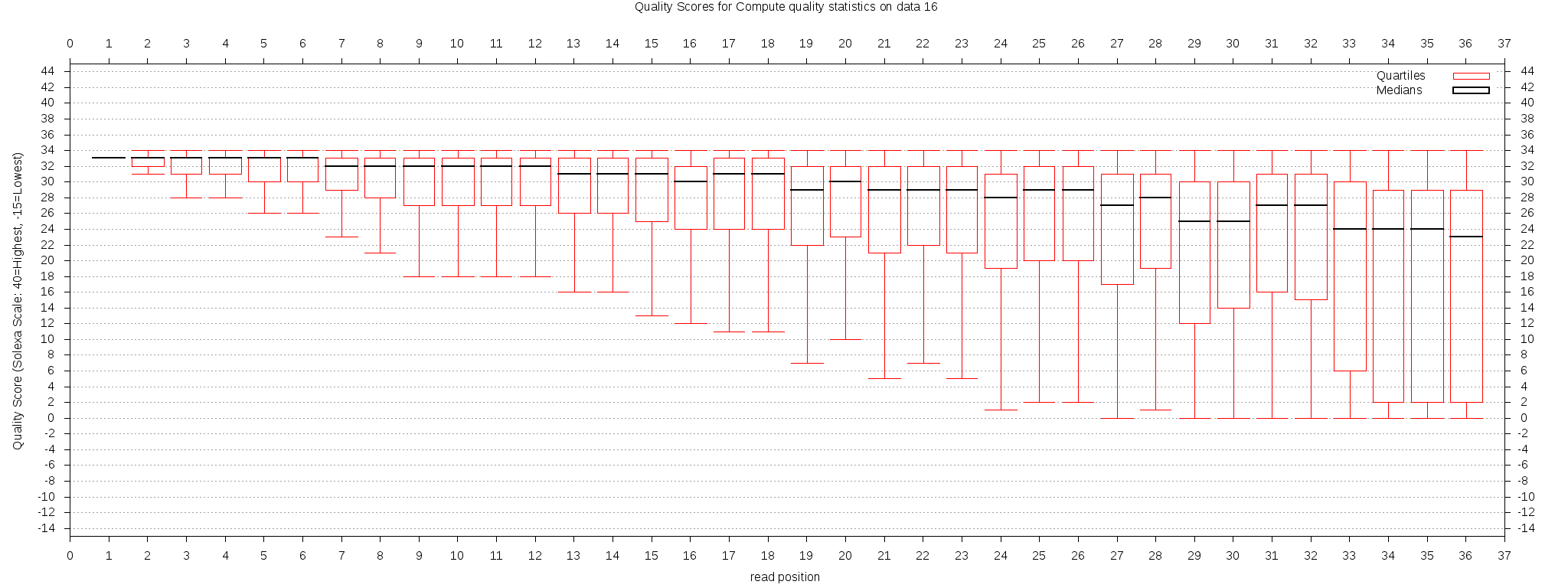
Figure 4 The quality of the test dataset. It appears that the quality of the reads are good overall before 25bp, while some reads have poor quality after that.
Case study: bivalent regions and the corresponding gene expression in guided differentiation
From multiple measured epigenomic data throughout guided differentiation process of mouse ES cells, we can find that certain epigenomic markers co-localize in the genome to create bivalent regions, whose epigenomic markers change during differentiation, together with the expression of their corresponding gene. This case study is based on the work from Xiao et al.[6].
Because some of the tools used, it will be quite difficult to fully complete this case study under Windows platform.
We would use the mapped ChIP-seq data for activin-A-induced guided differentiation of E14 at day 0 and day 6 to test if H2AZ and H3K27me3 will co-localize regions that serve as "poised promoters" and are correlated to gene expression changes.
To test this, 4 datasets will be used in this case study:
The regions in question are the mouse genome windows that have ortholog sequences in human named "MmToHs".
(Notice that if you download the bed files from GEO, they have the strand as their 4th column. This is not compliant to BED 6 format. To convert the files to BED 6 format, we can use the following command:
awk '{printf "%s\t%s\t%s\tread\t.\t%s\n", $1, $2, $3, $4 }' input_BED > output_BED
After conversion, BEDTools will be able to recognize the strand correctly.)
Because the steps will take long time to complete with the full dataset, we have provided miniature datasets (only reads on chr19 is included) for demonstration purposes. Results from the full dataset will be used later after the time-dependent procedures.
The corresponding regions in question is MmToHs_chr19.
All the contents involving the miniature dataset only will be marked in the same way as this box.
Besides all the files mentioned above, we still need some additional files:
We will put all these files under a new directory to begin the study.
Some of the steps may be done in Galaxy instead of using command line programs or scripts.
All steps that can be done in Galaxy will be shown in boxes like this one. However, some steps may need customized Galaxy deployment, while the stock tools in Galaxy from PSU may need extra steps and/or not yield exactly the same result as is shown here.
Count the reads to get the profile of markers in all interested windows
Because all reads have a length of 100bp while the average length of library DNA is 250bp during library preparation, it will be better to extend the mapped reads to its length before using them in downstream analysis. To extend the reads, we can use the "slop" feature from BEDTools[7]:
for i in mouse_*d?.bed; do /ecg/src/bedtools-2.17.0/bin/bedtools slop -s -l 0 -r 150 -g mouse.mm9.genome -i ${i} > ${i%.bed}_extend.bed; done;
In Galaxy, we can use Operate on Genomic Intervals -> Get flanks to achieve the same result, in settings, choose "Around start" as region, "Downstream" as Location, 0 as offset and 250 as flank length.
Do this to extend all of the datasets.
By stacking reads onto the windows, we can know if a window on the genome was marked or not. BEDTools has an "annotate" feature that can be used to count the coverage of feature over windows. To count the coverage of all markers over MmToHs, we can use the following command:
/ecg/src/bedtools-2.17.0/bin/bedtools annotate -names H2AZ_d0 H2AZ_d6 H3K4me3_d0 H3K4me3_d6 -counts -i MmToHs -files mouse_H2AZ_d0_extend.bed mouse_H2AZ_d6_extend.bed mouse_H3K4me3_d0_extend.bed mouse_H3K4me3_d6_extend.bed > output.bed
In Galaxy stock tools, we can use BEDTools (under NGS TOOLBOX BETA) -> Count intervals in one file overlapping intervals in another file to achieve similar but not exactly the same result. When doing this, use MmToHs (or MmToHs_chr19 if using miniature datasets) as target and extended data files of each individual feature as source.
After that, you will need to merge all the output file together as one file. Rename it as output.bed (or output_chr19.bed if using miniature datasets), and proceed with the following steps.
The output file can be downloaded here.
For miniature dataset, the extension command is the same, the annotation command is:
/ecg/src/bedtools-2.17.0/bin/bedtools annotate -names H2AZ_d0 H2AZ_d6 H3K4me3_d0 H3K4me3_d6 -counts -i MmToHs_chr19 -files mouse_chr19_H2AZ_d0_extend.bed mouse_chr19_H2AZ_d6_extend.bed mouse_chr19_H3K4me3_d0_extend.bed mouse_chr19_H3K4me3_d6_extend.bed > output_chr19.bed
The output file for miniature dataset can be downloaded here.
Get the windows that have its status changed throughout the process
A simple way to decide whether the (H2AZ, H3K4me3) status of a certain window is (+, +), (+, -), (-, +) or (-, -) is to set up a threshold for each marker, while windows with higher-than-threshold coverage can be considered positive. Threshold can be chosen in various ways, for example, by generating a histogram of the marker. In this mini case study, we take 5 as the threshold for each timepoint to simplify the case.
This step can be done in various ways. We recommend to use some scripting language to automate the process. Here is an example script, find_changed_region.R written in R (The leading "#" of output file need to be removed to be properly loaded in R). To use the script, first launch R, change the working directory to the current directory, and use the following code:
source("find_changed_region.R")
find_changed_region("output.bed","H2AZ","H3K4me3",5,5,5,5)
# If R complains about something about "Error in matrix",
# please check if the leading "#" in "output.bed" has been removed.
In this case study, we will focus on the (+, +) -> (+, -) and (+, +) -> (-, +) regions. The former are "activated" during differentiation while the latter are "repressed", so they should be associated with genes that have increasing expression and decreasing expression, respectively.
The results will be written to the following files under the same directory:
(+, +) -> (+, -) regions (11->10): output.bed.H2AZ.H3K4me3.11TO10.txt
(+, +) -> (-, +) regions (11->01): output.bed.H2AZ.H3K4me3.11TO01.txt
For miniature dataset, the script for R is:
source("find_changed_region.R")
find_changed_region("output_chr19.bed","H2AZ","H3K4me3",5,5,5,5)
# If R complains about something about "Error in matrix",
# please check if the leading "#" in "output_chr19.bed" has been removed.
However, because it is better to conduct epigenomic study on a whole genome scale, the following steps will be carried out by the full dataset, instead of the miniature. If you used the miniature for the previous steps, you can download the regions from the full dataset above.
Get corresponding genes from the status-changing window
Here we can use Genomic Regions Enrichment of Annotations Tool (GREAT) to find the gene associated with the regions. GREAT is available at http://bejerano.stanford.edu/great/public/html/index.php [8] and currently support human (GRCh37 and GRCh36.1), mouse (mm9) and zebrafish genome.
By uploading the regions in interest, we are able to learn what gene is associated with the regions, together with the enrichment of corresponding GO terms, protein products and other information.
For the "poised promoter" regions here, we use 5kb upstream, 5kb downstream and up-to-5kb distal regions. Also to utilize known regulatory domains, we would let GREAT to include them in the analysis.
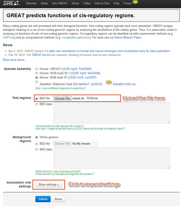
Figure 5 GREAT GUI. By uploading the poised promoter regions onto GREAT we are able to know associated genes.
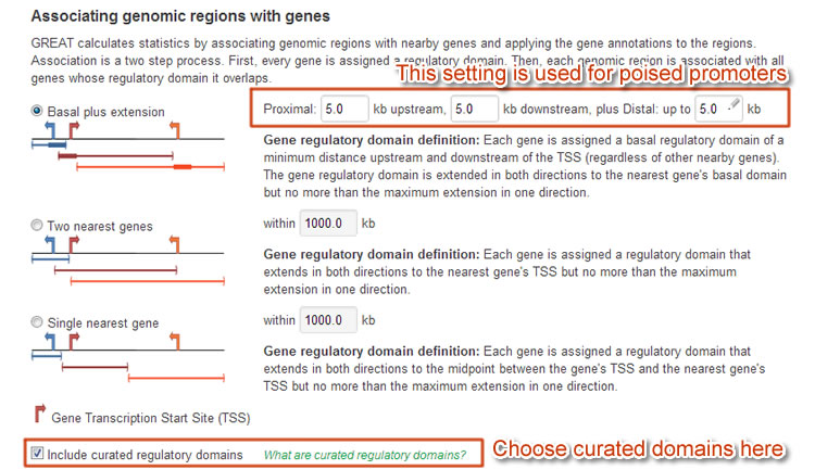
Figure 6 Settings for poised promoter
GREAT will generate the distance of the regions against the transcription starting site (TSS) of all associated genes, together with the enriched GO terms, protein product, phenotypes and other information.
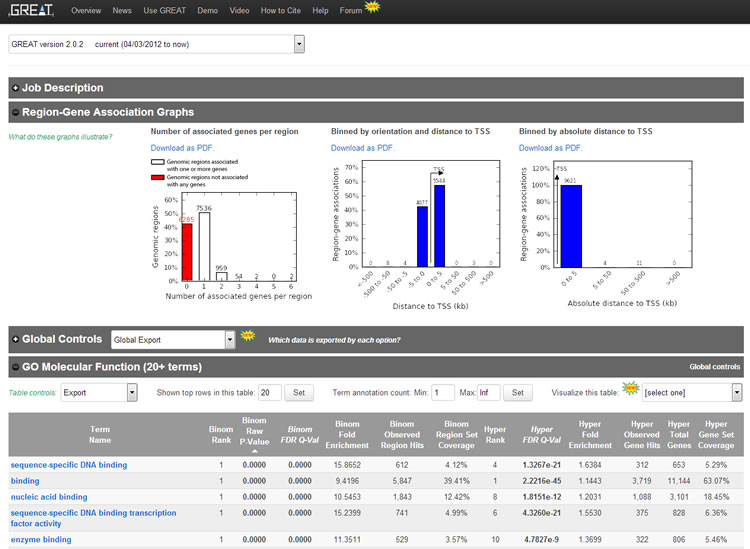
Figure 7 Overview of GREAT results.
Next we would use a temporal gene expression dataset to see if the regions really correlate with gene expression.
Filter the genes and plot expression
In this step, we will examine whether the regions are correlated to the expression change during differentiation.
First, we will need to save the associated gene list of every type (11->01 or 11->10) from GREAT. We will save them as "11-01.txt" and "11-10.txt" under the same directory of the expression dataset file "expression_MTC.txt".
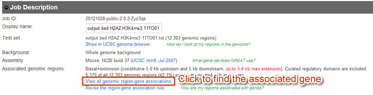
Figure 8 Use GREAT to download the associated gene list.
Then we can use the following script in R to generate the expression data of associated genes:
expression = read.table("expression_MTC.txt", sep = '\t', header = TRUE);
GREAT01 = read.table("11-01.txt", sep = '\t');
name01 = intersect(expression$gene_name, GREAT01[, 1]);
data01 = cbind(GREAT01[match(name01, GREAT01[, 1]),], expression[match(name01, expression$gene_name), ]);
GREAT10 = read.table("11-10.txt", sep = '\t');
name10 = intersect(expression$gene_name, GREAT10[, 1]);
data10 = cbind(GREAT10[match(name10, GREAT10[, 1]), ], expression[match(name10, expression$gene_name), ]);
With both expression data generated, we can either make a box plot, or a line plot of mean and standard deviation to see the expression trends. Both will show that the 11->01 regions (poised promoters that get "turned on" during differentiation) are associated with genes that have increasing expression level, while 11->10 regions with genes that have decreasing expression.
To make a box plot, we can use the following command:
boxplot(data01$FPKM_d0, data10$FPKM_d0, data01$FPKM_d4, data10$FPKM_d4, data01$FPKM_d6, data10$FPKM_d6, ylim = c(0, 70), pars = list(pch = '.'), col = c("grey", "tan"), ylab="RPKM", axes=FALSE, at=c(1.1,1.9,3.1,3.9,5.1,5.9), frame.plot=TRUE);
legend("topleft", c("11 -> 01","11 -> 10"), fill=c("grey","tan"));
axis(2);
axis(1, at=c(1.5, 3.5, 5.5), labels=c("Day 0","Day 4","Day 6"));
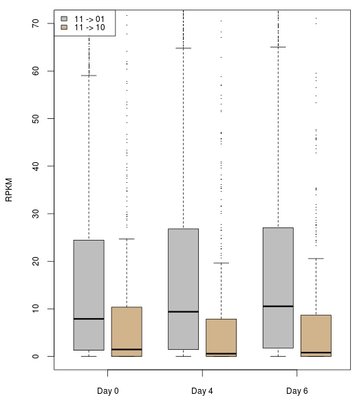
Figure 9 Box plot of genes associated with 11->01 (grey) and 11->10 (tan) regions. It shows that 11->01-region-associated genes have a trend of increasing expression while 11->10-region-associated genes have a decreasing trend.
To make a line plot with mean and sd of every time point, we can use the following command:
Error_plot <-function (Mean,Sd)
{
  len=length(Mean)
  lab=c("day0","day4","day6","day0","day4","day6")
  plot(1:3,Mean[1:3],ylim=c(min(Mean-Sd),max(Mean+Sd)),ylab="FPKM",xlab='',type='n',axes=FALSE)
  axis(1,1:len,lab[1:len])
  lines(1:3,Mean[1:3],type='b',col="grey",pch=16,lwd=2)
  lines(1:3,Mean[4:6],type='b',col="tan",pch=16,lwd=2)
  axis(2)
  arrows(1:3,(Mean+Sd)[1:3],1:3,(Mean-Sd)[1:3],angle=90,code=3,length=0.1,col="grey")
  arrows(1:3,(Mean+Sd)[4:6],1:3,(Mean-Sd)[4:6],angle=90,code=3,length=0.1,col="tan")
  legend("right", c("11 -> 01","11 -> 10"), pch=16, lty="solid", lwd=2, col=c("grey","tan"))
}
m1=colMeans(data01[,9:11])
m2=colMeans(data10[,9:11])
mean=c(m1,m2)
sd1=sd(data01[,9:11])/sqrt(dim(data01)[1])
sd2=sd(data10[,9:11])/sqrt(dim(data10)[1])
sd=c(sd1,sd2)
Error_plot(mean,sd)
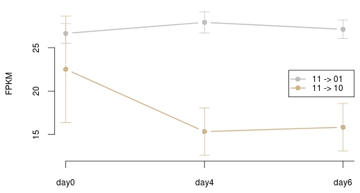
Figure 10 The mean and standard deviation of genes associated with 11->01 (grey) and 11->10 (tan) regions.